我找到了一种解决方案,可以为各种输入提供合理的结果。我首先拟合一个模型——一次到约束的低端,然后再到高端。我将这两个拟合函数的平均值称为“理想函数”。我使用这个理想函数来推断约束结束的左侧和右侧,以及在约束中的任何间隙之间进行插值。我定期计算理想函数的值,包括所有约束,从左边的函数接近零到右边的接近一。在约束处,我根据需要裁剪这些值以满足约束。最后,我构造了一个遍历这些值的插值函数。
我的 Mathematica 实现如下。
首先,几个辅助函数:
(* Distance from x to the nearest member of list l. *)
listdist[x_, l_List] := Min[Abs[x - #] & /@ l]

(* Return a value x for the variable var such that expr/.var->x is at least (or
   at most, if dir is -1) t. *)
invertish[expr_, var_, t_, dir_:1] := Module[{x = dir},
  While[dir*(expr /. var -> x) < dir*t, x *= 2];
  x]
这是主要功能:
(* Return a non-decreasing interpolating function that maps from the
   reals to [0,1] and that is as close as possible to expr[var] without
   violating the given constraints (a list of {x,ymin,ymax} triples).
   The model, expr, will have free parameters, params, so first do a
   model fit to choose the parameters to satisfy the constraints as well
   as possible. *)
cfit[constraints_, expr_, params_, var_] :=
Block[{xlist,bots,tops,loparams,hiparams,lofit,hifit,xmin,xmax,gap,aug,bests},
  xlist = First /@ constraints;
  bots = Most /@ constraints; (* bottom points of the constraints *)
  tops = constraints /. {x_, _, ymax_} -> {x, ymax};
  (* fit a model to the lower bounds of the constraints, and
     to the upper bounds *)
  loparams = FindFit[bots, expr, params, var];
  hiparams = FindFit[tops, expr, params, var];
  lofit[z_] = (expr /. loparams /. var -> z);
  hifit[z_] = (expr /. hiparams /. var -> z);
  (* find x-values where the fitted function is very close to 0 and to 1 *)
  {xmin, xmax} = {
    Min@Append[xlist, invertish[expr /. hiparams, var, 10^-6, -1]],
    Max@Append[xlist, invertish[expr /. loparams, var, 1-10^-6]]};
  (* the smallest gap between x-values in constraints *)
  gap = Min[(#2 - #1 &) @@@ Partition[Sort[xlist], 2, 1]];
  (* augment the constraints to fill in any gaps and extrapolate so there are
     constraints everywhere from where the function is almost 0 to where it's
     almost 1 *)
  aug = SortBy[Join[constraints, Select[Table[{x, lofit[x], hifit[x]},
                                              {x, xmin,xmax, gap}],
                                        listdist[#[[1]],xlist]>gap&]], First];
  (* pick a y-value from each constraint that is as close as possible to
     the mean of lofit and hifit *)
  bests = ({#1, Clip[(lofit[#1] + hifit[#1])/2, {#2, #3}]} &) @@@ aug;
  Interpolation[bests, InterpolationOrder -> 3]]
例如,我们可以拟合对数正态、正态或逻辑函数:
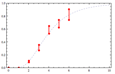
g1 = cfit[constraints, CDF[LogNormalDistribution[mu,sigma], z], {mu,sigma}, z]
g2 = cfit[constraints, CDF[NormalDistribution[mu,sigma], z], {mu,sigma}, z]
g3 = cfit[constraints, 1/(1 + c*Exp[-k*z]), {c,k}, z]
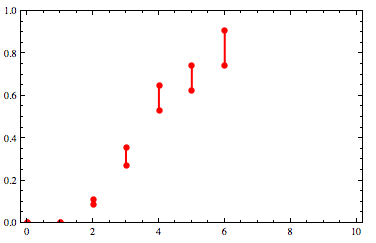
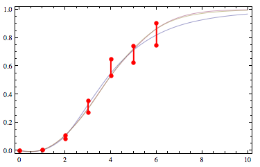
这是我的原始示例约束列表的样子:

(来源:yootles.com)
正态和逻辑几乎在彼此之上,对数正态是蓝色曲线。
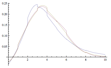
这些都不是很完美。特别是,它们不是很单调。这是导数的图:
Plot[{g1'[x], g2'[x], g3'[x]}, {x, 0, 10}]

(来源:yootles.com)
这表明缺乏平滑度以及接近零的轻微非单调性。我欢迎对此解决方案进行改进!


