我已经编写了一些代码来使用网格图形来做到这一点。这里有一个例子:https ://qdrsite.wordpress.com/2016/06/26/pies-on-a-map/
这里的目标是将饼图与地图上的特定点相关联,而不一定是区域。对于这个特定的解决方案,有必要将地图坐标(纬度和经度)转换为 (0,1) 比例,以便将它们绘制在地图上的适当位置。网格包用于打印到包含绘图面板的视口。
代码:
# Pies On A Map
# Demonstration script
# By QDR
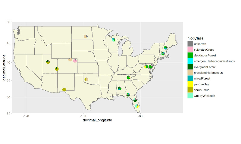
# Uses NLCD land cover data for different sites in the National Ecological Observatory Network.
# Each site consists of a number of different plots, and each plot has its own land cover classification.
# On a US map, plot a pie chart at the location of each site with the proportion of plots at that site within each land cover class.
# For this demo script, I've hard coded in the color scale, and included the data as a CSV linked from dropbox.
# Custom color scale (taken from the official NLCD legend)
nlcdcolors <- structure(c("#7F7F7F", "#FFB3CC", "#00B200", "#00FFFF", "#006600", "#E5CC99", "#00B2B2", "#FFFF00", "#B2B200", "#80FFCC"), .Names = c("unknown", "cultivatedCrops", "deciduousForest", "emergentHerbaceousWetlands", "evergreenForest", "grasslandHerbaceous", "mixedForest", "pastureHay", "shrubScrub", "woodyWetlands"))
# NLCD data for the NEON plots
nlcdtable_long <- read.csv(file='https://www.dropbox.com/s/x95p4dvoegfspax/demo_nlcdneon.csv?raw=1', row.names=NULL, stringsAsFactors=FALSE)
library(ggplot2)
library(plyr)
library(grid)
# Create a blank state map. The geom_tile() is included because it allows a legend for all the pie charts to be printed, although it does not
statemap <- ggplot(nlcdtable_long, aes(decimalLongitude,decimalLatitude,fill=nlcdClass)) +
geom_tile() +
borders('state', fill='beige') + coord_map() +
scale_x_continuous(limits=c(-125,-65), expand=c(0,0), name = 'Longitude') +
scale_y_continuous(limits=c(25, 50), expand=c(0,0), name = 'Latitude') +
scale_fill_manual(values = nlcdcolors, name = 'NLCD Classification')
# Create a list of ggplot objects. Each one is the pie chart for each site with all labels removed.
pies <- dlply(nlcdtable_long, .(siteID), function(z)
ggplot(z, aes(x=factor(1), y=prop_plots, fill=nlcdClass)) +
geom_bar(stat='identity', width=1) +
coord_polar(theta='y') +
scale_fill_manual(values = nlcdcolors) +
theme(axis.line=element_blank(),
axis.text.x=element_blank(),
axis.text.y=element_blank(),
axis.ticks=element_blank(),
axis.title.x=element_blank(),
axis.title.y=element_blank(),
legend.position="none",
panel.background=element_blank(),
panel.border=element_blank(),
panel.grid.major=element_blank(),
panel.grid.minor=element_blank(),
plot.background=element_blank()))
# Use the latitude and longitude maxima and minima from the map to calculate the coordinates of each site location on a scale of 0 to 1, within the map panel.
piecoords <- ddply(nlcdtable_long, .(siteID), function(x) with(x, data.frame(
siteID = siteID[1],
x = (decimalLongitude[1]+125)/60,
y = (decimalLatitude[1]-25)/25
)))
# Print the state map.
statemap
# Use a function from the grid package to move into the viewport that contains the plot panel, so that we can plot the individual pies in their correct locations on the map.
downViewport('panel.3-4-3-4')
# Here is the fun part: loop through the pies list. At each iteration, print the ggplot object at the correct location on the viewport. The y coordinate is shifted by half the height of the pie (set at 10% of the height of the map) so that the pie will be centered at the correct coordinate.
for (i in 1:length(pies))
print(pies[[i]], vp=dataViewport(xData=c(-125,-65), yData=c(25,50), clip='off',xscale = c(-125,-65), yscale=c(25,50), x=piecoords$x[i], y=piecoords$y[i]-.06, height=.12, width=.12))
结果如下所示: